- Overview
- Background for newcomers
- Why pre-register
- How the question was chosen
- Related work
- Design
- Methods
- Pipeline
- Registration
- Power
- Results
- Robustness
- Exploratory
- Post hoc checks (not registered)
- Implications and open questions
- Deviations
- Limitations
- Reproduce
- What review caught before registration
- Use of AI tools
- References
Overview
| At a glance | |
|---|---|
| Question | Why did 29 of 334 ACOs end their Shared Savings Program agreements early in 2022 to reset their benchmarks, and did renewing change their spending? |
| Data | Public CMS files, 2014-2026: ACO enrollment, performance-year results, county spending and county assignment (40 files, 40 MB) |
| Design | Pre-registered on OSF before any outcome was read; group comparisons, a decision model and a difference-in-differences estimate, with decision rules fixed in advance |
| Methods | Bayesian bootstrap, stratified permutation tests, Bayesian logistic regression with measurement error, direct-simulation tests, difference-in-differences with an equivalence rule, conventional comparisons |
| Tools | Python, dbt on DuckDB, PyMC, statsmodels, uv; an interactive dashboard in plain JavaScript; a marimo notebook |
| Finding | Early renewers' regions spent more relative to their benchmarks, but they were also beating their benchmarks, so on average a reset would not have raised them; no detectable change in spending afterward |
| Reproduce | About 10 minutes to download the data and run the tests; about 18 hours to rerun every stage (Reproduce) |
| Manuscript | The journal-style write-up, its tables and figures, the results files and the post hoc scripts: stharrold/mssp-paper-2026, archived on Zenodo (DOI 10.5281/zenodo.23737045)1 |
| Video | "Resetting the Target Early": a 17-minute narrated explainer for a general audience (watch it here or on YouTube); its slides as PDF and PowerPoint |
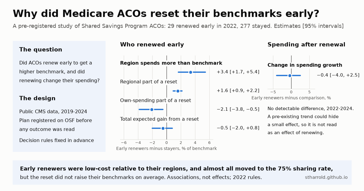
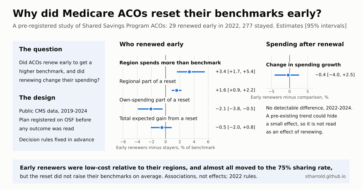
The visual abstract (select it for the full-size image) is drawn from the same results files as the dashboard
(report/visual_abstract.py; SVG).
In the Medicare Shared Savings Program2 (MSSP), an accountable care organization3 (ACO) earns a share of the savings when its patients' spending comes in below a benchmark. As of January 1, 2026, 511 ACOs served 12.6 million assigned Medicare beneficiaries (CMS fast facts4). The benchmark is reset at the start of each agreement period5 from the ACO's own recent spending, pulled toward its region's. An ACO can end its agreement early and start a new one6, which resets the benchmark early. Of the 334 ACOs whose agreements began July 1, 2019 or January 1, 2020, 29 ended them early and started new ones on January 1, 2022; 277 stayed in their agreements and 28 left the program (from the enrollment files7).
This post asks why they did, and what renewing changed:
- Who chose to reset, and why (H1-H3). Did early renewers stand to gain from a reset because their regions spent more than their benchmarks (the primary test), because their own spending had run high, or because renewing was the only way into the track that shares 75% of savings8 without waiting for the agreement to end or leaving the program?
- Spending after renewal (H4). Did early renewers' spending change afterwards, relative to ACOs that had not yet renewed? A difference-in-differences estimate.
Terms used throughout:
- PY: performance year, the calendar year over which CMS measures an ACO's spending against its benchmark.
- Benchmark years (BY1-BY3): the three years before an agreement starts, whose spending sets the new benchmark.
- BASIC and ENHANCED tracks: BASIC has five levels, A to E. Levels A and B are one-sided (the ACO shares savings only), and C to E are two-sided (it also repays part of any losses). ENHANCED is two-sided with the highest sharing rate.
- Glide path: BASIC's schedule for moving an ACO up a level each year, toward two-sided risk.
The analysis plan was registered on OSF Registries (DOI 10.17605/OSF.IO/C53W9)9 before any outcome value was read, together with the analysis code, which was written and tested on synthetic data10 first. Every result below is reported, whatever it shows; changes made after registration are listed separately under Deviations.
In short. The primary test found what the plan calls "evidence for the reset motive beyond past savings": early renewers' regions spent 3.4 percentage points of benchmark more than stayers' regions, relative to their current benchmarks (95% credible interval 1.7 to 5.4, p < 0.001). That is not a larger expected gain. Early renewers were beating their benchmarks by more than stayers, with savings rates about 2 points higher, and by the approximation a reset would on average have lowered both groups' benchmarks (by about 1.6% for early renewers and 1% for stayers): early renewers stood to gain more from the regional adjustment and to lose more on their own spending. A check added after the study, against CMS's own published 2022 benchmarks, agrees: early renewers' new benchmarks came in 1.3% below their old ones on average. So the primary result says more about early renewers being low-cost relative to their regions than about a higher benchmark. In the decision model, renewing early was more likely with a higher regional pull and a higher BASIC level. Early renewers' spending growth in PY2022-PY2024 did not differ detectably from that of ACOs not yet renewed (-0.4%, -4.0% to +2.5%); a continuing pre-period difference in trends cannot be ruled out, so this is not read as an effect of renewing.
In plain English.
- Early renewers were in regions that spend more. The ACOs that reset early tended to be in places where Medicare spends more per patient, relative to the ACO's own benchmark, than the places stayers were in: about 3.4% of the benchmark more, or roughly $385 per patient per year at the median benchmark of $11,312 in PY2021 (the PY2021 results file11). A reset pulls the benchmark toward the region's spending, so these ACOs had more to gain from that part of it.
- But they were already beating their benchmarks. They spent further below their targets than other ACOs did. A reset also resets the target to the ACO's own recent spending, so for most of them that part would have cut the benchmark. By the study's estimate the two parts roughly cancel, and a reset would not have raised the average early renewer's benchmark. CMS's own numbers, checked afterwards, agree: early renewers' new 2022 benchmarks were about 1.3% below their 2021 ones on average.
- ACOs at higher BASIC levels renewed early more often. ACOs already at BASIC's higher, two-sided levels (C to E) were more likely to renew early; 16 of the 27 BASIC-track early renewers were at the top level, E. Renewing was their way into ENHANCED, which keeps 75% of savings, so the pattern fits an interest in the higher sharing rate, but it cannot be told apart from the regional motive, because both came with the same choice.
- Spending afterward looked about the same. Early renewers' spending growth in 2022-2024 was close to that of ACOs that had not renewed. The data rule out a drop of more than about 4% or a rise of more than about 2.5%, but a difference in trends that began before renewal could still hide a smaller effect, so this is not read as "renewing had no effect".
- What this means. ACOs that reset early were, on average, low-cost relative to their regions, and almost all of them gained a higher sharing rate. A reset was not a simple way to get a higher benchmark. Read as an interpretation rather than a test, the pattern fits the sharing rate as the draw better than the benchmark, and that is the trade CMS built into the rules12, under which moving from BASIC to ENHANCED during an agreement required renewing early, and so a reset.
- These are the 2022 rules. Benchmarks for agreements starting in 2024 or later give ACOs credit for past savings and soften the cut for an ACO that spends more than its region, so the same trade-off may not hold for an ACO renewing today (see Limitations).
The study in a 17-minute video
"Resetting the Target Early" tells the same story for a general audience, with a made-up example of how a reset works
and no statistics background needed. It is narrated, with captions, and is also on the blog's YouTube channel,
Data Science Demos. The video loads from YouTube only when you press play (see the
privacy page). The slides are also a download: PDF (fonts embedded, opens anywhere) or PowerPoint
(the editable original, with the narration in its speaker notes; its headings fall back to another font where Domine
is not installed). The video is built by the code in video/, and the transcript below comes from the
deck's speaker notes through report/video_slides.py.
Transcript (one paragraph per slide)
- In January 2022, twenty-nine groups of doctors and hospitals did something odd. They quit their Medicare contracts early and signed new ones, which reset the targets Medicare uses to decide whether they earn a share of savings. By Medicare's own numbers, checked after the study, two thirds of them ended up with a lower target. A more difficult one. So why do it? I ran a study to find out, and I wrote down the rules before I looked at the data. Here's what I found.
- I'm Samuel Harrold, and this is a pre-registered study of public Medicare data. You don't need any background in healthcare or statistics to follow along.
- First, a familiar idea. Imagine your boss sets next year's sales targets from what you sold this year. You crush it, and your reward is a harder target. Do too well today, and tomorrow gets tougher. Economists call this a ratchet, because it only clicks one way. Medicare has its own version of this, and it's the key to the whole puzzle.
- Here's the program. It's called the Medicare Shared Savings Program, and the groups in it are called ACOs, short for accountable care organizations. That's the one acronym you need. An ACO is just a group of doctors and hospitals. Medicare adds up the total cost of care for each group's patients. If it comes in under a target, the group keeps part of the savings. It's big: five hundred eleven groups, covering about twelve point six million people with Medicare.
- Let's use one made-up example with round numbers. Medicare sets this group's target at eleven thousand dollars per patient per year. The group's patients actually cost ten thousand five hundred. That's five hundred dollars saved per patient, or seven and a half million dollars across fifteen thousand patients. How much does the group keep? On the common track, up to half: about three point seven five million. On the top track, called ENHANCED, seventy-five percent: about five point six million. Same savings, almost two million dollars more. Remember that gap.
- Now the catch. The target doesn't stay put. When a group signs a new contract, Medicare rebuilds the target, starting from the group's own recent spending. Our group spent ten thousand five hundred, so its new target starts there: five hundred dollars lower. Save money, and your next target gets harder. That's the ratchet. If that were the whole story, no successful group would ever want to reset. But there's a second part.
- Next, Medicare nudges the target toward what similar patients cost in the group's region. Say comparable patients nearby cost twelve thousand dollars. That's fifteen hundred more than our group spent. The first time, the rules move the target thirty-five percent of the way toward the region. Thirty-five percent of fifteen hundred is five hundred twenty-five dollars. So a group in an expensive area gets a boost. How much room a group has for that boost is what I'll call the regional pull. It's the main thing this study measured.
- Let's add the two parts. Start at ten thousand five hundred, from the group's own spending. Add five hundred twenty-five for the region. The new target is eleven thousand and twenty-five dollars. The old one was eleven thousand. Almost exactly where it started. The penalty for saving and the bonus for an expensive area cancel out. I picked these numbers on purpose. Keep this picture in mind, because the real data looked a lot like it.
- So here's the puzzle. Contracts normally last five years, but a group could quit early and immediately sign a new one. Renewing early did two things at once. First, it reset the target sooner. Second, for groups on the main track, it was the only way to move up to the top track, ENHANCED, before their contract ran out. That's the one that keeps seventy-five percent of savings, though it also means owing back up to seventy-five percent of any losses. Two changes, one decision.
- I looked at three hundred thirty-four groups whose contracts started in mid-2019 or January 2020. Twenty-nine renewed early, on January first, 2022. I'll call them early renewers, in orange. Two hundred seventy-seven stayed put: the stayers, in blue. And twenty-eight left the program. So what made those twenty-nine different? One caution: twenty-nine is a small number, and I'll be upfront about what that limits.
- There are two suspects. Suspect A: a better target. Maybe a reset would have raised their target, giving them more room to earn savings. Suspect B: a bigger share. Maybe they wanted the seventy-five percent track, and renewing early was the only door. The trouble is, both came with the same decision, so no test can fully pull them apart. But one of these suspects doesn't hold up the way you'd expect. Before we get there, here's how I made sure I couldn't fool myself.
- Before I looked at a single spending number, I wrote down every question I'd ask, every test I'd run, and the exact words I'd use for each possible result. Then I posted it publicly. It's called pre-registration. Think of calling your shot in pool: eight ball, corner pocket. Why bother? Because these files are public, and if you slice data enough ways, something will look exciting just by chance. Researchers fall into that trap without meaning to. Calling the shot means you can tell a planned test from a lucky find.
- And you can check it. The plan was registered on OSF, the Open Science Framework, which stamps the time itself, on October twenty-sixth, 2026. The analysis code refused to open any spending file until that registration existed. And I tested everything first on fake data with known answers planted in it. Reviews of the plan before registration also caught a real flaw: my first main test was quietly just a restatement of past savings. Catching that before the plan was locked, instead of after, is the whole point.
- One more check before the results. Medicare doesn't publish what a group's target would have been after a reset, so I rebuilt it from public files. I tested the rebuild on one hundred one groups where Medicare did publish the answer. It passed the bar I'd set in advance: it ranked groups almost exactly the way Medicare did, and the typical miss was one point six percent.
- Now, how to read the results. Each one is a best guess, the dot, and a range of plausible values, the bar. Ask one question: does the bar cross zero? Here, the best guess is plus three point four, and the whole bar sits above zero. That's a clear difference. Here, the best guess is minus half a point, and the bar crosses zero. That doesn't prove there's no difference. It means we can't tell it apart from none. You'll see both of these again in a minute.
- Finding one, the main question. Were early renewers in places where care costs more than their target? Yes. The gap was bigger than for stayers, by about three point four percent of the target. That's roughly three hundred eighty-five dollars per patient per year. It passed the test I set in advance, and by my own rule it counts as evidence for suspect A, the better target. Case closed? Not quite. That's only one of the two parts.
- Finding two. Early renewers were already beating their targets, by more than stayers. In 2020 they saved about six point four percent of their target, against four point six for stayers, and the gap held in 2021 too. That comes straight from Medicare's own reports. And remember the catch: a reset restarts from your own spending. For strong savers, that part cuts the target. So one part helps them more, and the other hurts them more.
- Here's what happens when you put them together. The blue bar is the regional boost. Early renewers stood to gain a little over one and a half points more than stayers. The orange bar is the own-spending catch. They stood to lose about two points more, because they'd been saving more. Add them up, and you get the grey bar: about minus half a point, with a range that crosses zero. The boost and the penalty cancel. It's our eleven thousand and twenty-five example, in real data. After the study, I checked what actually happened, using Medicare's published 2022 targets. Early renewers' new targets came in about one point three percent lower on average, and two thirds of them went down. That check wasn't in the original plan, so I'm labeling it as an add-on. But it agrees. So on average, a reset didn't hand these groups a better target.
- Finding four is about suspect B, the bigger share. Of the twenty-seven early renewers on the main track, twenty-six moved up to the seventy-five percent track. And sixteen of them were already at the main track's top level, one short step away. In a model of who renewed, being at a higher level stood out, along with the regional pull. One caution: that model rests on just twenty-four groups, so trust the direction, not the exact size.
- Finding five: did renewing change spending? Compared with groups that hadn't renewed yet, early renewers' spending growth was about the same: minus zero point four percent, with a range from minus four to plus two and a half. So we can rule out a drop bigger than about four percent, or a rise bigger than about two and a half. But I can't call it "no effect." I had only one earlier period to compare trends, during COVID, and a trend that started before renewal could hide a small effect. My plan said not to call it an effect in that case, so I don't.
- So what can this study say? It shows which groups chose to reset, what a reset stood to do to their targets, and that spending didn't shift by more than a few percent. What it can't say: that renewing caused anything, since groups chose for themselves; which suspect was the real reason; or what any of this cost Medicare.
- So why did they hit reset? On average, not for a better target. By the later check, their targets mostly went down. But nearly all of them got the bigger share, and many were one step away. For a low-cost group that's already saving, keeping seventy-five percent instead of fifty percent can be worth more than a small drop in the target. That's my reading, not a tested result. But it fits how Medicare wrote the rules: if you wanted the bigger share mid-contract, a reset came with it.
- A few limits. The biggest: these are the 2022 rules. For contracts starting in 2024 or later, Medicare gives groups credit for past savings, so the trade-off may look different today. The numbers are small. My rebuilt targets are good for averages, rough for single groups. Thirty-nine smaller groups couldn't be measured, because Medicare hides tiny counts for privacy. And there was only one earlier period, during COVID.
- A quick disclosure. An AI tool, Claude Code from Anthropic, proposed this topic and drafted the analysis plan, the code, and most of the written post, and separate AI instances reviewed them. I chose among its options, registered the plan, ran the analysis, and I'm responsible for the results. The slides and script for this video were drafted with Claude's help too. Because the plan was public before any result existed, you can check it either way.
- Three things to remember. One: the groups that reset early were low-cost compared with their neighbors, and already saving more. Two: a reset didn't raise their targets on average. The bigger seventy-five percent share is the likelier draw. Three, and this goes far beyond Medicare: write down your rules before you look, and people can trust your answer, even when it's messy.
- If you want to dig in, the full write-up, the registered plan and the code are all linked in the description. And if you've ever had a target ratchet up on you, tell me about it in the comments. Thanks for watching.
The narration says renewing early was the only way onto the higher-sharing track. More exactly, it was the only way without waiting for the contract to end or leaving the program, as Design explains.
Background for newcomers
Four short primers for readers new to the program or the methods; each opens on a click, and experienced readers can skip them.
How the Shared Savings Program works, with a worked example
An ACO is a group of doctors and hospitals that agrees to be measured on the total Medicare spending of the patients assigned to it. CMS sets a benchmark: the spending it expects per patient per year. If the ACO's patients cost less, and the ACO meets quality standards and saves more than a minimum rate, it keeps a share of the savings. On the BASIC track that share is up to 40% (one-sided levels A and B, which never owe money) or 50% (two-sided levels C to E, which also repay part of any losses). On ENHANCED it is up to 75%, with up to 75% of losses (42 CFR 425.605, 425.610).
A made-up example, ignoring risk adjustment, trends and caps:
- The benchmark is $11,000 per patient and the ACO's 15,000 patients cost $10,500 each: $500 saved per patient, $7.5 million in all. At a 50% sharing rate the ACO receives about $3.75 million; at 75%, about $5.6 million.
- At the next agreement the benchmark is reset. The new one starts from the ACO's own recent spending, about $10,500, so the own-spending part of a reset lowers it by $500: beating the benchmark today makes the next one harder.
- It is then adjusted toward the region. If comparable patients in the ACO's region cost $12,000, the benchmark moves part of the way there: with the phase-in weight of 35% that applies the first time (it rises to 50% later), by 0.35 x ($12,000 - $10,500) = $525. That is the regional part, and the regional pull measures how much room there is for it.
- The new benchmark is about $10,500 + $525 = $11,025, almost the same as before. This is the pattern the study found for early renewers: the regional gain and the own-spending loss roughly cancel.
Agreements last five years. Early renewal ends one early and starts a new one, which resets the benchmark sooner and, for a BASIC ACO, is the way into ENHANCED. More: CMS's program page2 and the rule, 42 CFR 425.601.
Association and causation: what the methods can and cannot show
Statistics cannot prove that one thing caused another. A study design can make a causal claim credible, under assumptions it states and checks. The effect of renewing early on an ACO is the difference between what happened and what would have happened had the same ACO not renewed, and that second outcome is never observed. A randomized experiment solves this by making the groups alike on average. Here ACOs chose for themselves, so the ones that renewed may differ in ways that also affect spending (selection).
- H1-H3 are associations. They describe which ACOs chose to renew early, and say nothing about what renewing caused.
- H4 uses difference-in-differences. It compares the change in spending of early renewers with the change for ACOs that had not yet renewed. That is an effect only if, without renewal, both groups' spending would have changed in parallel (parallel trends), ACOs did not change behavior in anticipation, and one group's choice did not affect the other's spending. Earlier years can test parallel trends only weakly, and here there is one earlier change, so the plan required an equivalence condition before reading H4 as an effect. It did not hold.
- Pre-registration guards against a different problem: trying many analyses and reporting the one that works. Fixing the analyses and decision rules first means a reader can trust that the reported tests were not chosen after seeing the results.
More, all free online: Cunningham's Causal Inference: The Mixtape, Huntington-Klein's The Effect, and Hernán and Robins's Causal Inference: What If.
Bayesian and frequentist statistics, side by side
The two schools answer different questions about the same data.
- A frequentist p-value asks: if there were no real difference, how often would chance alone produce a difference at least as large as the one observed? Here chance is simulated directly: the early-renewer labels are shuffled 10,000 times, and the p-value is the share of shuffles with a difference at least as large. A confidence interval is a range built by a procedure that captures the true value in 95% of repeated studies.
- A Bayesian posterior describes what is plausible about the true value after seeing the data, given a model and a prior (what was assumed before). A 95% credible interval is a range with 95% probability of holding the true value, under that model. In this study the priors are mild: on the log-odds scale, Normal(0, 1) says large effects are unlikely, which keeps the estimates stable with only 24 early renewers in the decision model. A second fit with wider Student-t priors checks that the results do not depend on that choice.
The study uses both on purpose. Estimates and their uncertainty are Bayesian. The yes-or-no decisions use p-values against thresholds fixed in the registration, because a rule written in advance is easy to check. The conventional (frequentist) versions are reported beside them, and every verdict agrees, so the conclusions do not hinge on the choice of school.
More: VanderPlas's Frequentism and Bayesianism: A Python-driven Primer (free) and McElreath's Statistical Rethinking.
How to pre-register your own observational study
This study's plan (PREREGISTRATION.md13) can serve as a template. Its sections are the ones a registry
expects:
- Background and hypotheses: each with its predicted direction and its role (primary, secondary, descriptive).
- Data: the sources, and what you have and have not already seen.
- Sample and groups: exact inclusion rules, and how missing or hidden values are handled.
- Variables: how each is built, and how any approximation is validated before it is used.
- Analysis plan: every estimate and test, robustness checks, and what is exploratory.
- Power: what effect sizes the data can detect.
- Decision rules: the exact wording for each possible result, written before any result exists.
- Deviations: how later changes will be logged.
Register it with an independent registry that records the time itself (see OSF's guide to registrations), keep the code that reads outcome data locked until then (this study's outcome lock is described under Why pre-register), and log every later change before using its results.
Why pre-register
The CMS public use files14 used here are public. Anyone analyzing them can try many specifications and report the one that works, often without meaning to (Simmons, Nelson and Simonsohn 201115). A pre-registration fixes the question, the variables, the tests and the decision rules before the outcomes are seen, so a reader can tell confirmatory results from exploration (Nosek et al. 201816).
Two details make that claim checkable here:
- An independent timestamp. Git commit dates can be set by hand, so the plan was registered on
OSF Registries, which records the time itself. The plan file's sha256 and the registered
code commit are recorded in
REGISTRATION.md17, so the repository copy can be matched to the registered one. - An outcome lock in the code. Every data file is hashed before it is read10. A file whose hash matches a
performance-year results file or a county spending file could not be opened until
REGISTRATION.mdexisted. There was no bypass flag. Before registration only the enrollment files7, the CMS data dictionaries (for example the PY2021 results dictionary11) and the regulation text18 were used, plus the column names (not the values) of the outcome files, to write the code. The enrollment files include each ACO's track and BASIC level, so H3's prediction for the BASIC level was written with those data available: pre-registered, but not blind to them.
How the question was chosen
The question in this post was the fourth candidate. The first three were dropped at the design stage, using only the regulation and the enrollment files:
- Downside risk. The program's "glide path" moves ACOs into two-sided risk on a schedule19, which looked like a natural experiment. The regulation showed that the timing is partly chosen: ACOs choose the level they start at, can move up faster20, and could pause the advance for 2021 and 2022; from 2023, an ACO still in one-sided Level A or B could stay there for the rest of its agreement. The enrollment files7 showed that only about 10-28% of ACOs were in two-sided risk in the years the schedule called for it. Not a usable treatment.
- The benchmark ratchet. Do ACOs spend less once their spending starts counting toward the next benchmark? In the enrollment data, benchmark-year status is collinear with how long the ACO has been in its agreement, so the effect cannot be separated from tenure. Kept only as a descriptive table.
- A correction. An early tabulation found 139 ACOs leaving their benchmark-year schedule at the 2022 transition, and an unverified inference treated them all as early renewers. Accounting for the optional one-year extension21 of agreements that began in 2018 (from the 2020 interim final rule22) showed that only 29 renewed early into a January 1, 2022 agreement.
Those 29 became the question. A first version asked only whether they had lower savings rates. That was too narrow to explain anything, so the plan became explanatory, with two motives that predict different things.
Related work
Five strands of earlier work bear on this study. Only one, an industry report rather than peer-reviewed research, looks at early renewal itself.
-
The same early renewers, in an industry report. Milliman's report on 2022 results tabulates gross savings rates for the ACOs that rebased early in 2022, the same 29 as here (11 that were in the program before Pathways to Success and 18 that joined in 2019 or 2020). Both groups had higher savings rates in 2020 and 2021 than comparable ACOs that did not rebase, and each of the 11 moved from BASIC levels C to E into ENHANCED (Smith et al. 202423). A Milliman case study models the same choice for one hypothetical ACO (Milliman 202524).
-
Rebasing creates a ratchet. The rules for setting an ACO's benchmark at renewal weaken its incentive to save, and the old weights on the benchmark years even rewarded higher spending just before a new agreement (Douven, McGuire and McWilliams 201525). This is the ratchet effect that arises whenever targets are set from past performance (Weitzman 198026), and a 2026 dissertation found MSSP savings rates 40% higher in years whose spending did not enter a future benchmark (Cappello 202627). That is one reason the H4 design guards against anticipation and mean reversion.
- ACOs differ widely from their regions. Even after case-mix adjustment, ACOs' spending varies widely relative to local fee-for-service spending, so moving benchmarks toward regional averages shifts them unevenly (Rose, Zaslavsky and McWilliams 201628). That variation is what the regional pull measures, and why its case-mix adjustment matters (see Limitations).
- Benchmarks drive who participates. After regional spending entered benchmarks in 2017, participation shifted toward providers whose spending was low relative to their region (Lyu, Chernew and McWilliams 202329), ACOs whose effective benchmark fell, because of a separate 2017 change in assignment rules, were 7 percentage points more likely to leave (Chen and McWilliams 202530), and ACOs with a positive regional adjustment were about 70% less likely to exit (Cappello 202627). In a Medicare bundled-payment program made voluntary for half of its hospitals after 2 mandatory years, hospitals that could gain without changing their behavior were more likely to opt in, which the authors call selection on levels (Einav et al. 202231). The primary result here is the same kind of selection, in when to reset rather than whether to join or leave.
- The 2019 rules changed participation decisions. Under Pathways to Success, for the first time more ACOs left the program than joined it: 73 exits against 65 entrants in 2019 (Ying et al. 202332). ACOs that had achieved savings were more likely to stay, a borderline result (odds ratio 1.76, 95% interval 0.99 to 3.09), and so were ACOs with higher spending, which the authors read as a sign that administrators "needed to see enough room" to make their savings target, the same consideration as the reset motive here. ACO leaders described reassessing potential savings against losses in light of the benchmark changes (Ying et al. 202433). Of the Track 1 ACOs facing renewal in 2019, 40% left, at a projected cost of up to $396.8 million in lost savings by 2022 if that rate continued (Moloci et al. 202134).
How these results fit, in plain English.
- Agrees with (industry data): Milliman found that the ACOs that renewed early in 2022 had been saving more, and that those already in the program before 2019 moved to ENHANCED. This study finds the same, and adds why the savings matter: beating the benchmark makes a reset cost more.
- Agrees with: earlier work found that ACOs pick their moment using the benchmark. They joined when the regional formula favored them (Lyu and colleagues), and they left when their effective benchmark fell (Chen and McWilliams). This study finds the same behavior in a new choice, when to reset: early renewers were the ACOs whose regions spent more relative to their benchmarks.
- Fits with, though that evidence is weak: after the 2019 rules, ACOs that were already saving money were more likely to stay in the program, a borderline result whose interval includes no effect (Ying and colleagues). Early renewers here were also savers, beating their benchmarks by more than other ACOs. But that same success meant a reset would have cut the own-spending part of their benchmark, so the simple story "ACOs reset to get a higher benchmark" does not fit them on average.
- Consistent with: earlier work showed that comparing an ACO with its region is sensitive to how patients' health is adjusted for (Rose and colleagues). Here too, the size of the regional difference doubles without that adjustment.
- Cannot confirm or rule out: the worry that rebasing rewards spending more just before a new agreement (Douven and colleagues). Early renewers' spending growth afterward showed no detectable difference, but the design could not separate an effect from a trend that started before renewal.
- Does not address: what departures or early renewals cost Medicare (Moloci and colleagues estimated the cost of departures); this study does not estimate costs.
This study adds a pre-registered analysis of which ACOs used the option to reset their benchmark early, and of what a
reset stood to give them, measured with public data. The Milliman reports were found later, by a critical review of the
manuscript1. The search used Google Scholar Labs (three queries on 2026-10-27, one
rejected as too broad), and its questions, raw results and per-paper summaries are saved in the study's
research/ folder.
Design
Groups
The base population is the 334 ACOs in the enrollment files7 whose agreements began July 1, 2019 or January 1, 2020 (plan section 313). Both cohorts' agreements run to December 31, 2024 (42 CFR 425.200(b)(4)(ii)21 and (b)(5)), so a January 1, 2022 agreement start means an early renewal: an ACO that terminated its agreement35 and immediately entered a new one (425.20, "renewing ACO"6).
| Group | 2019-07-01 cohort | 2020-01-01 cohort | All |
|---|---|---|---|
| Early renewers | 11 | 18 | 29 |
| Stayers | 159 | 118 | 277 |
| Left after PY2021 | 19 | 9 | 28 |
Two motives, and why the savings rate cannot separate them
- The reset motive. A new benchmark would be higher than the current one.
- The sharing-rate motive. An ACO in the BASIC track36 cannot move to the ENHANCED track during an agreement period (2018 rule12), so renewing early was the only way in without waiting for its agreement to end or leaving the program. ENHANCED shares 75% of savings8 and up to 75% of losses. In the enrollment files7, 26 of the 27 early renewers that were in BASIC moved to ENHANCED; no stayer could, since the move is barred within an agreement period.
The expected benchmark gain from a reset has two parts: an own-spending part (how the ACO's recent spending compares with its current benchmark) and a regional part (the adjustment toward the region5). The own-spending part is close to a restatement of the savings rate. Writing out the regional adjustment shows that it contains the own-spending part too, with a negative sign. With phase-in weight \(w\), before capping,
where "pull" is the regional pull defined below and "own" the own-spending component, so the regional part is also tied to past savings. The primary test therefore uses the regional pull: how far the region's spending, adjusted to the ACO's case mix the way CMS adjusts it5, sits above the ACO's current benchmark,
where \(R_e\) is the risk-adjusted regional spending for enrollment type5 \(e\) (ESRD, disabled, aged/dual, aged/non-dual), \(s_e\) the ACO's share of person-years of that type, and \(B\) its current per-capita benchmark. It has no term for the ACO's own benchmark-year spending, though it is not free of the ACO's own data: \(B\) was set from the ACO's earlier spending, and \(R_e\) is adjusted with the ACO's own risk scores (see Limitations). An ACO can be beating its own benchmark and still stand to gain from a reset because its region spends more; that is the part of the reset motive a savings rate cannot show.
Hypotheses
As registered (plan section 1.313):
| Hypothesis | Role | |
|---|---|---|
| H2b | Early renewers had a larger regional pull than stayers | Primary |
| H2a | Early renewers had a larger own-spending component | Secondary (close to H1 restated) |
| H1 | Difference in PY2020 savings rate | Descriptive context, no motive attributed |
| H3 | Among BASIC-track ACOs, the probability of renewing rises with regional pull, own-spending component and a higher BASIC level | Decision model |
| H4 | Early renewal changed per-capita spending in PY2022-PY2024 | Effect estimate, two-sided |
H1-H3 describe who chose to reset and why; they are associations, not effects. H4 estimates the effect of a bundled package (a new benchmark, for almost all a move to ENHANCED, and a change in which years count toward the next benchmark) and cannot separate its parts.
Building the expected gain from public data
CMS does not publish what an ACO's benchmark would have been had it reset. The plan rebuilds it from 42 CFR 425.6015 in six steps (section 4.313), which come down to four parts:
- the equally weighted mean5 of the ACO's per-capita spending in the three benchmark years (PY2019-PY2021), risk-adjusted and restated to the latest year's risk scores (CMS's methodology specifications, version 1037, section 4.1.2, step 3), and trended to 2021 dollars with the national-regional blend;
- risk-standardized regional spending from the county files38, weighted by where the ACO's beneficiaries live5 (from the assigned-beneficiaries-by-county files39) and adjusted to the ACO's case mix;
- the regional adjustment with the phase-in weights5 and caps;
- and the shares that combine the four enrollment types5.
Because several steps can only be approximated from public files, the approximation was validated before it was used: rebuilt for the regular renewers whose 2022 benchmarks CMS does publish (in the results files11; 101 of the 111 eligible; 10 lack either the rebuilt or the published benchmark), with a pass rule fixed in the plan (section 4.413: Spearman correlation at least 0.80, median absolute percentage error at most 5%). Early renewers were kept out of the validation sample, and the 2022 results file was filtered as it was loaded, so validation could not reveal their actual reset.
Methods
Estimates and significance
Every confirmatory estimate is Bayesian, and significance is measured by resampling: the null distribution is simulated rather than looked up (an accessible introduction is VanderPlas's "Statistics for Hackers"; video40, slides).
- Group comparisons (H1, H2a, H2b, H4). The estimate is the difference in means, early renewers minus stayers, within each cohort and averaged with weights proportional to the early renewers in each cohort. Its posterior is a Bayesian bootstrap (Rubin 198141): 10,000 draws of Dirichlet(1, ..., 1) weights over the ACOs in each cohort-by-group cell.
-
Significance by stratified permutation. Early-renewer labels are shuffled within cohort 10,000 times, and the estimate is recomputed on each shuffle. The two-sided p-value is
\[p = \frac{1 + \#\{\,|\hat\theta_\text{shuffled}| \ge |\hat\theta_\text{observed}|\,\}}{1 + 10{,}000}\]
Adding 1 to both counts treats the observed labels as one of the shuffles, so the p-value is never zero (Phipson and Smyth 201042). The resampling p-value decides, by rules written before the results (below). When it and the credible interval disagree, both are reported.
H3: a Bayesian decision model with measurement error
A logistic regression of early renewal on the three core predictors (regional pull, own-spending
component, higher BASIC level) and five adjustment factors (cohort, size, revenue category, assignment method, first
or later agreement), fit with PyMC43 (NUTS44, 4 chains of 2,000 draws; plan section 5.413).
Continuous predictors are scaled by two standard deviations (Gelman 200845), so each coefficient is a
log-odds difference per 2 SD. With 24 events (27 eligible early renewers, 3 missing a predictor) and 9
parameters, the Normal(0, 1) priors keep the estimates stable, so a second fit with Student-t priors, the scale Gelman et al. 200846 recommend for scaled predictors but with 3 rather than 1 degree of freedom, is reported for sensitivity. A Firth-penalized logistic regression
(Firth 199347, fit with firthmodels48) with the core predictors and cohort is always run
beside it, and decides H3 only if the Bayesian model fails its convergence checks49.
The own-spending component is an approximation, so it enters as a latent true value observed with error,
with \(\sigma_v\) set by the validation step before the model is fit (4.38 percentage points, from CMS's own
benchmark-year spending for the validation sample; validation.json17).
Shuffling labels in a model with several predictors would test "nothing matters", not "this factor matters given the others". Each core predictor is instead tested by direct simulation under the reduced model (a parametric bootstrap): fit the model without that predictor, simulate 10,000 sets of outcomes from its posterior, refit the full model to each, and compare the observed coefficient with that null distribution. That is about 40,000 MCMC refits, which took 17 hours on 5 cores.
H4: difference-in-differences with an equivalence rule for pre-trends
The outcome is log per-capita spending. For each ACO,
and the H4 estimate is the same cohort-weighted difference in means as above, applied to \(\Delta\). Comparison ACOs are those not yet renewed: a stayer's years after it renews into a 2023 or 2024 agreement are dropped, following the not-yet-treated idea of Callaway and Sant'Anna (2021)50 (plan section 5.813).
The main threat is selection on the outcome's own path: if early renewers renewed after unusually high spending, their spending could fall afterwards by mean reversion alone. There is only one pre-period change (PY2020 to PY2021, both affected by COVID-19), and with about 29 treated ACOs a non-significant pre-trend test proves little (Roth 202251). So H4 counts as an effect only if an equivalence condition holds (the logic of an equivalence test52): the pre-trend interval, scaled to the distance between period midpoints, must rule out a trend difference large enough to produce the estimate. A trend-adjusted estimate (the pre-period slope carried forward, the exactly linear special case of the restrictions of Rambachan and Roth 202353) is reported beside it, along with propensity-score-weighted (Rosenbaum and Rubin 198354; Callaway and Sant'Anna 202150), risk-adjusted, balanced-panel and single-cohort versions.
Conventional methods, side by side
For comparison, and not used for any decision (plan section 5.713): Welch t-tests (Welch 194755) and OLS with HC2 robust errors (MacKinnon and White 198556) for H1, H2a and H2b; maximum-likelihood logistic regression for H3 (statsmodels57); and two-way fixed effects with an event study, errors clustered by ACO, for H4. An agreement table puts each registered verdict next to the conventional one; for H2a and H2b the registered counterpart is OLS with HC2 errors, and the Welch t-test is shown beside it.
Decision rules
Fixed before the results (plan section 713). For H2b: p < 0.05 and positive means "early renewers' regions spent more relative to their current benchmarks, evidence for the reset motive beyond past savings"; p < 0.05 and negative is evidence against it; otherwise "no detectable difference", reported with the credible interval and the minimum detectable effect. No test here can rule the sharing-rate motive in or out, because in these data it is bundled with the reset in a single choice.
What was simulated, and when
Simulated data played no part in forming the hypotheses. Three kinds of data were used, at three stages:
| When | Data | Used for |
|---|---|---|
| Before registration | The regulation, the enrollment files, the data dictionaries, and the outcome files' column names (not their values) | Choosing the question and writing the hypotheses (How the question was chosen) |
| Before registration | Synthetic data, made up by ratchet/synthetic.py10 |
Writing and testing the pipeline before any outcome could be read |
| After registration, before any confirmatory estimate | Simulations calibrated to the real data | The power analysis (plan section 613) and the H3 direct-simulation tests |
The synthetic values are invented, not fitted to CMS data: no CMS outcome value was viewed to write the generator.
It builds a small stand-in (270 ACOs in the two cohorts and 80 regular renewers, in 3 states of 15 counties) with
lognormal spending, and it copies the real files' quirks: column names that change between years, * suppression
markers, date formats, and early-renewer rows the loader must drop. It also plants known answers. Early renewal is
made more likely with a higher regional pull and own-spending component (logistic coefficients 1.0 and 0.6 per SD),
and spending is 4% lower after renewal. The tests10 check that the SQL matches an independent NumPy
computation of every constructed variable, that the decision model recovers a planted direction on made-up data,
and that H4 recovers the -4% to within 0.015 log points.
The power analysis uses real spreads, read after registration as the plan allows: the PY2016-PY2018 savings-rate SD
for H1, the stayers' SDs of the regional pull and own-spending component for H2, and the SD of the pre-period
spending change for H4 (power.json17).
Pipeline
The pipeline is in analysis/mssp-benchmark-ratchet/10, linked here as registered (commit a4064f5):
- Data snapshot. Every CMS file used is listed with its size, sha256 and URL in
data-snapshot.tsv10, and each hash is checked before the file is read. The files come from four CMS datasets: ACO enrollment7, performance-year results11, county expenditures and risk scores38 and assigned beneficiaries by county39. - dbt for the SQL. The constructed variables are a dbt58 project on DuckDB59
(dbt-duckdb, in
dbt/10): 28 models, one per derived table, in three tagged stages, with schema and data tests (unique keys, accepted values, components adding to the gain, shares summing to one, no early renewer in the validation load). Python loads every raw table after its hash check, so dbt never reads a file directly. - Two implementations. A synthetic-data generator10 writes made-up files with the real file and column names and computes the constructed variables independently in NumPy. The tests require the SQL to match it, and every stage runs end to end on synthetic data, including the recovery of a planted -4% effect in H4.
- Staged runner10. Each stage refuses to start until the outputs it depends on exist: validate, then power, then confirm and robustness (both need only validation and power, and ran at the same time), then did, conventional and exploratory. So the power analysis was committed before any confirmatory estimate. The robustness results were committed first, about 17 hours before the confirmatory ones, and were read only together with them, primary test first.
- Reproducible environment. uv60 with a lockfile; PyMC,
firthmodelsandstatsmodels57 are pinned inuv.lock, and every refit has its own seed from a fixed seed sequence61 (parallel streams), so results do not depend on the number of processes. They do vary slightly between runs, within simulation error, because the analysis table is read without a fixed row order (see Reproduce).
Writing the code before registering found gaps in the plan while it could still change: column names that drift
between years (ACO_Num and ACO_ID, Sav_Rate and Sav_rate), how calibration splits between the gain's two
parts, how "below its region" is compared, and the per-refit seeds.
Registration
| Item | Value |
|---|---|
| Registration | osf.io/c53w9, DOI 10.17605/OSF.IO/C53W9 |
| Registered | 2026-10-26 13:22:16 UTC, public, no embargo |
| Plan | PREREGISTRATION.md v0.6, sha256 d0e374c8b493eb2f2fa7da1c0d8cbe46745a601233f11a81d2b2be73c402e8f2 |
| Code | commit a4064f5, zip sha256 4c98d76a586151ab608851c69217a5ddb6b394201643a3de89a839bb1f659cd4 |
The zip can be rebuilt from the repository and checked against the registered copy:
git archive --format=zip a4064f5 analysis/mssp-benchmark-ratchet pyproject.toml uv.lock | shasum -a 256
The attached Markdown file is the authoritative copy of the plan; OSF's summary field holds a plain-text version (checked through the OSF API before submission).
Power
Computed after registration and committed before any confirmatory estimate, as the plan requires
(section 613; power.json17). Minimum detectable effects at 80% power, two-sided alpha
0.05, for 29 vs 277 ACOs:
| Test | Minimum detectable effect |
|---|---|
| H1 savings rate | 2.7 percentage points (simulated power 80.4%) |
| H2b regional pull | 2.5 percentage points |
| H2a own-spending component | 1.8 percentage points (0.55 SD) |
| H4 spending change | 3.8 log points (a change of +3.9% or -3.7%) |
H3 is underpowered. At a true log-odds difference of 0.5 per 2 SD, the 95% interval excludes zero in only 17% (regional pull), 0% (own-spending component) and 14% (BASIC level) of simulated datasets. If the true effects were about that size, an "undetermined" H3 verdict was the expected outcome. Power was simulated only at 0.5.
Results
In the order the plan fixes: the validation that decides how the own-spending component is used, the primary test,
then H2a, H1, H3 and H4. Each verdict quotes the decision rule written before the results
(plan section 713). Every number comes from the results files in results/17, each of which
records the commit it ran at.
Validation of the benchmark approximation
Passed. For the 101 regular renewers whose 2022 benchmarks CMS publishes (of 111 eligible; 10 lack either the rebuilt
or the published benchmark), the rebuilt benchmark had a Spearman correlation of 0.94 with the actual one and a
median absolute percentage error of 1.6% (the rule: at least 0.80 and at most 5%). The regression of actual on
rebuilt had slope 0.944 and intercept 664, inside the plan's 0.9-1.1 range for the slope, so no calibration was
applied. By phase-in step of the regional adjustment: 62 ACOs at the first step (Spearman 0.93, error 2.0%) and 39
at the second (0.96, 0.9%). The step-1 check of the own-spending part against CMS's own benchmark-year spending gave
Spearman 0.95 and error 1.4% (101 ACOs), and its error SD sets \(\sigma_v\) = 4.38 percentage points
(validation.json17). The own-spending component is therefore used as registered, not as
exploratory.
These checks are on benchmark levels, which vary widely across ACOs. The own-spending component is a difference, and its estimated error (\(\sigma_v\) = 4.38 points) is larger than its spread among stayers (SD 3.3), so at the level of one ACO it is mostly noise. H2a, the total expected gain and the offset argument below rest on it; the H1 savings rates, which CMS reports directly, are the firmer evidence that early renewers were beating their benchmarks.
Who renewed early (H2b, H2a, H1)
Early renewers minus stayers, within cohort and weighted by early renewers per cohort
(confirm.json17). Expected-gain variables are in percentage points of the current benchmark (1 point
is 1% of the benchmark, about $113 per patient per year at the median PY2021 benchmark of $11,312); savings rates are
in percentage points.
| Comparison | Early renewers minus stayers | 95% credible interval | p | Minimum detectable effect |
|---|---|---|---|---|
| H2b regional pull (primary) | +3.4 | 1.7 to 5.4 | < 0.001 | 2.5 |
| H2a own-spending component | -2.1 | -3.8 to -0.5 | 0.003 | 1.8 |
| H1 savings rate, PY2020 | +1.9 | 0.7 to 3.3 | 0.010 | 2.7 |
| H1 savings rate, PY2021 | +1.6 | 0.2 to 3.1 | 0.033 | 2.7 |
| Total expected gain (descriptive) | -0.5 | -2.0 to 0.8 | 0.33 | |
| Regional component (descriptive) | +1.6 | 0.9 to 2.2 | < 0.001 |
26 early renewers and 241 stayers for the expected-gain variables, 29 and 277 for H1 (see Limitations for the exclusions).
- H2b (rule 1): the regional pull, how far the region's case-mix-adjusted spending sits above the ACO's current benchmark. p < 0.05 and positive: "early renewers' regions spent more relative to their current benchmarks, evidence for the reset motive beyond past savings". The difference is larger than the minimum detectable effect, which was computed for 29 vs 277 ACOs and so is slightly understated for the 26 vs 241 compared. In unweighted means, the early renewers' regions spent 5.0 points above their benchmarks, the stayers' 1.8 points.
- H2a (rule 2, which applies rule 1's wording to the own-spending component): how the ACO's own recent spending compares with its current benchmark (negative when it spends below it). p < 0.05 and negative; in rule 1's terms adapted to this component, their own spending was lower relative to their benchmarks, contrary to the reset motive. Early renewers were beating their benchmarks by more than stayers. H2a is close to H1 restated, so it is not counted as separate evidence.
- H1, descriptive (rule 3). Early renewers had higher savings rates in both years. No motive is attributed to the sign. (The PY2020 results file11 stores savings rates as fractions and the PY2021 file as percents; both are shown here in percentage points.)
The tables and the dashboard label these outcomes "supported" (H2b) and "contradicted" (H2a), shorthand for rule 1's two directions.
The two parts of the gain point in opposite directions and offset: the regional component is larger for early
renewers, the own-spending component smaller, and the total expected gain does not differ. On average a reset would
have lowered both groups' benchmarks, by the approximation: in unweighted means the own-spending and regional parts
sum to -5.3 + 3.7 = -1.6 points for early renewers and -3.2 + 2.2 = -1.0 for stayers (exploratory.json17).
That follows from the savings: rebasing to an ACO's own spending lowers the benchmark of any ACO that has been
beating it. Weighted by the phase-in weight, the pull difference is 1.6 points (Exploratory), the
same as the regional component's. So the evidence is about where early renewers stood relative to their regions, not
about a larger expected gain from resetting; a check against CMS's published 2022 benchmarks bears this out
(Post hoc checks). That is the
configuration the plan described before any outcome was read (section 1.313): an ACO "can be beating its own
benchmark and still stand to gain from a reset because its region spends more". As the plan also says (rule 8), no
test here can rule the sharing-rate motive in or out.
H3: the decision model
206 BASIC-track ACOs, 24 of them early renewers (3 early renewers and 27 stayers excluded for a missing predictor;
confirm.json17).
Coefficients are log-odds differences per 2 SD, or for the BASIC level between levels C-E and A-B. A log-odds
difference of 1.34 multiplies the odds of renewing early by about 3.8.
| Predictor | Posterior mean | 95% credible interval | Direct-simulation p | Verdict |
|---|---|---|---|---|
| Regional pull | 1.34 | 0.44 to 2.30 | 0.002 | supported |
| Own-spending component | -0.05 | -2.01 to 1.92 | 0.19 | undetermined |
| Higher BASIC level (C-E) | 1.34 | 0.38 to 2.31 | 0.003 | supported |
| 2020-01-01 cohort | 0.63 | -0.24 to 1.51 | adjustment | |
| Log assigned beneficiaries | 0.45 | -0.49 to 1.36 | adjustment | |
| High revenue | -0.53 | -1.69 to 0.59 | adjustment | |
| Prospective assignment | -0.77 | -1.79 to 0.19 | adjustment | |
| Later agreement | -0.67 | -1.62 to 0.31 | adjustment |
- Verdicts (rule 4). The regional pull and a higher BASIC level are supported; the own-spending component is undetermined. The overall test (the largest absolute core coefficient against its simulated null) gives p = 0.004. Adjustment factors are estimates only.
- What the BASIC level means. The plan's rationale for it is a smaller step to two-sided risk under ENHANCED
(section 1.313): 16 of the 27 BASIC-track early renewers were already at Level E in 2021, BASIC's
highest level, for whom ENHANCED was a short further step (
exploratory.json17). That bears on the sharing-rate motive at least as much as on the reset motive, and the two cannot be separated here. The level is also partly chosen: ACOs experienced with performance-based risk could enter BASIC only at Level E, if not ENHANCED (42 CFR 425.600(d)19), so it partly records past risk experience. - Checks. The model met its convergence checks on the first fit (largest R-hat62 1.001, smallest bulk effective sample size 6,661, no divergences). The Student-t fit needed its one registered rerun, then converged, and agrees: regional pull 1.65 (0.53 to 2.87), BASIC level 1.63 (0.53 to 2.85), own-spending component -0.56 (-9.98 to 7.36). In the direct-simulation tests, 0.34-0.43% of the refits did not converge. Before seeing the outcomes, the priors implied a median 17% of ACOs renewing early (95% range 1% to 70%). In posterior predictive checks the observed 24 early renewers fall inside the replicated 95% range (14 to 37), and in the top predicted decile 57% renewed against 45% predicted.
- The own-spending coefficient is the prior. Its interval is the prior's 95% range, because the measurement error (\(\sigma_v\) = 4.38) is larger than the variable's spread among stayers (SD 3.3): the model can learn almost nothing about it. Without the measurement-error model (a robustness check) it is -0.64 (-1.51 to 0.23).
- Read the sizes with care. The power analysis gave H3 a 17% (pull) and 14% (BASIC level) chance of detecting a log-odds difference of 0.5. An estimate that passes a test with power that low is likely to overstate the true effect (a "type M" error, Gelman and Carlin 201463), so the directions are the result, and coefficients near 1.3 (odds ratios near 4) are probably too large.
H4: spending after renewal
29 early renewers and 276 comparison ACOs not yet renewed (one stayer has no spending value in any post-period
year; did.json17). The outcome is the change in log per-capita spending from
PY2020-PY2021 to PY2022-PY2024, shown as a percent difference in spending growth.
| Estimate | Early renewers minus comparison | 95% credible interval | p |
|---|---|---|---|
| H4 | -0.4% | -4.0% to +2.5% | 0.78 |
| Pre-trend (PY2020 to PY2021) | +0.7% | -2.3% to +4.9% | 0.58 |
| Trend-adjusted | -4.0% | -12.0% to +2.7% | 0.14 |
- Verdict (rule 5). "No detectable difference"; the minimum detectable effect is 3.8 log points (about 3.9%).
- Not read as an effect. The pre-trend test is not evidence against parallel trends (p = 0.58), but the equivalence condition does not hold: the scaled pre-trend bound, 2.41 years times 0.048, is 0.115 log points (a log difference; about 12%), far above the H4 estimate of 0.004. The condition needed an estimate above 0.115 log points, about 12% and three times the minimum detectable effect. With one pre-period, that threshold was a property of the design, fixed at registration: for any estimate near zero, the rule could only end in "not read as an effect". A trend difference of the size the pre-period allows could hide an effect in either direction. So H4 is reported as a difference in spending changes that cannot be told apart from a continuation of a pre-period difference in trends.
- What the data do bound. Under parallel trends, the H4 interval (-4.0% to +2.5%) rules out a drop in spending growth of more than about 4% or a rise of more than about 2.5%. The trend-adjusted interval (-12.0% to +2.7%) is too wide to be informative.
-
Attrition. The plan requires it by group and year (section 4.513), and it is uneven:
Group and status PY2022 PY2023 PY2024 Early renewers (29): included 29 28 25 Early renewers: left the program 0 1 1 Early renewers: renewed again 0 0 3 Stayers (277): included 276 222 162 Stayers: left the program 0 46 72 Stayers: renewed (no longer "not yet renewed") 0 8 42 Stayers: no spending value 1 1 1 By PY2024, 115 of 277 stayers (42%) had dropped out of the comparison, against 4 of 29 early renewers (14%). Exits are unlikely to be random: the ACOs that left after PY2021 had the lowest savings rates (see Exploratory). The balanced panel, ACOs with all five years, is the check on this: -1.6% (-5.6% to +1.6%), p = 0.30.
Registered and conventional methods
Every verdict agrees with its conventional counterpart (reported only; it would not have changed a decision;
conventional.json17):
| Claim | Registered | Conventional |
|---|---|---|
| H2b | supported (p < 0.001) | supported: OLS with HC2 errors +3.3 (1.3 to 5.4), p = 0.001 |
| H2a | contradicted (p = 0.003) | contradicted: OLS with HC2 errors -2.1 (-3.8 to -0.4), p = 0.018 |
| H3 regional pull | supported (p = 0.002) | supported: logistic odds ratio 4.0 (1.2 to 13.4), p = 0.024 |
| H3 own-spending component | undetermined (p = 0.19) | undetermined: odds ratio 0.53 (0.19 to 1.44), p = 0.21 |
| H3 higher BASIC level | supported (p = 0.003) | supported: odds ratio 4.8 (1.5 to 15.6), p = 0.009 |
| H4 | no detectable difference (p = 0.78) | two-way fixed effects -1.5% (-5.4% to +2.4%), p = 0.44 |
The conventional p-values are mostly larger than the resampling ones, but no verdict changes. The Welch t-tests agree too: H2b +3.2 (1.1 to 5.3), p = 0.004; H2a -2.1 (-3.9 to -0.2), p = 0.028.
Interactive results
Loading the interactive results...
Results notebook
The main results tables and figures are also in a marimo64
notebook
(report/results_notebook.py17). It reads the results files through the dashboard's data
builder and recomputes nothing: provenance (each results file's commit and sha256), validation, the group
comparisons, H3, H4, the agreement table, robustness and exploratory results. This post is the authoritative report;
some details added after the critical review (such as the H4 attrition table) are only here. The notebook page loads
marimo's front end from jsDelivr, so the OSF project also holds a PDF and a
Jupyter notebook with its outputs saved, which need no CDN. The files below were exported on 2026-10-27, after the
review changed the H4 wording, and replaced the first upload on OSF, which keeps the earlier versions in each file's
history:
| File (on OSF) | sha256 |
|---|---|
results.html |
65fe501e57ceae5eba3fc76533f81a1047771c3ef7ff87db20f72559b93c877a |
results.ipynb |
761f0306fa2b4a5a3ab373b72a71da4f510192810e2b198e6687fbc9f6ee228f |
results.pdf |
32bc555e591b253d7b7aa142a4946bc69e2566fd402a88c5cd9686c69f341630 |
Robustness
The robustness checks of plan sections 5.513 and 5.8 (robustness.json17
and did.json). The robustness stage ran alongside the confirmatory one, and its results were read only
together with the confirmatory results. They do not change the verdicts; the dashboard above shows each one next to its confirmatory estimate.
- H2b keeps its direction in every check. Difference in medians +2.8 (p < 0.001); 2020-01-01 cohort only +3.7 (p = 0.001); unadjusted county spending +6.9 (p = 0.002); Bayesian regression with cohort only +2.1 (0.5 to 3.8) and with track, level and size added +2.2 (0.7 to 3.8). The size depends on the estimator: the regression estimates are below the minimum detectable effect and well below the +3.4 difference in means, which suggests a few large values among early renewers carry part of it, and the unadjusted version is twice as large.
- H2a is weaker by medians. -1.4, p = 0.085; the other checks keep it below zero with p < 0.05 (cohort only p = 0.043, benchmark years 2-3 only p = 0.012, complete cases p = 0.005), though the adjusted regression's interval reaches zero (-2.6 to 0.02).
- H1 is weaker with adjustment. By medians +1.4 points (p = 0.061), and in the adjusted regression +1.2 (-0.1 to 2.6).
- H3's directions hold, with two intervals at zero. The Firth regression gives the same verdicts (pull p = 0.004, BASIC level p = 0.006, own-spending p = 0.18). The pull coefficient's interval reaches zero with the 2020-01-01 cohort only (1.15, -0.02 to 2.39) and with unadjusted county spending (0.75, -0.02 to 1.56); the BASIC level's stays above zero in every check.
- H4 shows no detectable difference in any check. Risk-adjusted outcome +0.3% (p = 0.85), balanced panel -1.6% (p = 0.30), propensity-weighted -0.5% (p = 0.67, largest weight 0.83), 2020-01-01 cohort only -2.9% (p = 0.13), trend-adjusted -4.0% (p = 0.14).
Exploratory
Labeled exploratory in the plan (section 5.613; exploratory.json17): no predictions and no verdicts, and nothing here was used to choose
what is reported above.
- Other measures of the regional pull. Weighted by the phase-in weight \(w\), early renewers minus stayers is +1.6 (0.7 to 2.6); the capped regional component, +1.6 (0.9 to 2.2). Both are positive in H3 too.
- Census region65 adds nothing to the decision model: Midwest, South and West, each against the Northeast, all have intervals that include zero, and the pull and BASIC-level coefficients barely move (1.43 and 1.32).
- Leavers. The 28 ACOs that left after PY2021 had the lowest savings rates (mean 2.7 points in PY2020, against 6.4 for early renewers and 4.6 for stayers), and a regional pull (for 20 of the 28) similar to early renewers' on average (4.8 against 5.0) but much lower in the median (2.0 against 3.5).
- The two early renewers already in ENHANCED, for whom renewing could not raise the sharing rate, fall between the 26th and 68th percentile of stayers on every variable (savings rate at the 38th and 65th, regional pull at the 26th and 61st).
- Spending by agreement year rises for every group; early renewers from 2020 agreements started lower and stayed lower. As the design noted, benchmark-year status cannot be separated from tenure here, so this is description only.
Post hoc checks (not registered)
Added on 2026-10-27 and 2026-10-28, after every registered result had been read, in response to critical reviews of
the manuscript1. posthoc/validation_change.py and
posthoc/pull_savings.py66 reuse the registered pipeline's tables and estimator and change no
registered file; nothing here decides a hypothesis.
- Validation on the change scale. The registered validation checks benchmark levels, which vary widely across ACOs; the hypotheses concern differences of a few points. For the same 101 regular renewers, the rebuilt change from the PY2021 benchmark agrees only moderately with the actual one: Spearman 0.61, median absolute error 1.7 points, mean error -0.3, same sign for 80%. Group means hold up better than any one ACO's value.
- Early renewers' realized reset. CMS's published 2022 historical benchmarks for the 29 early renewers averaged 1.3% below their PY2021 benchmarks (median 1.5% below; 66% lower). For the 26 with both values, the rebuilt gain predicted -1.6 points on average, against -1.4 realized.
- The benchmark a year later. From PY2021 to PY2022 the updated benchmark, which includes the annual update, rose 3.1% for early renewers and 2.9% for stayers on average; within cohort the difference is 0.0 points (-2.0 to 2.2), p = 0.97.
- The regional pull and past savings. The pull is measured against the current benchmark, which was set from the ACO's own earlier spending, so it could be past savings by another name. Among the 267 early renewers and stayers with the variable, its rank (Spearman) correlation with the PY2020 savings rate is 0.45, with PY2021 0.23 and with the own-spending component -0.25 (stayers alone: 0.42, 0.23 and -0.25). The pull is related to past savings, but most of its variation is not.
Implications and open questions
For program design, the results suggest that the early-renewal option let ACOs choose when to reset. The ones that used it more often had regions that spent more relative to their benchmarks and were more often at higher BASIC levels, for whom ENHANCED was a short step. That is selection into an option the program created; it is not evidence that renewing changed spending. Three questions remain open:
- What did early renewal cost Medicare, through higher benchmarks or larger shared-savings payments? This study does not estimate it.
- Did the 2024 rules change who renews early? The prior savings adjustment and the limits on negative regional adjustments weaken the own-spending penalty that early renewers faced in 2022. 34 stayers renewed early into 2024 agreements under those rules, so the data to look are public.
- How much of the choice was the sharing rate rather than the benchmark? In these data the two came with the same decision; a period in which ACOs could move to ENHANCED without resetting would separate them.
Deviations
None affecting any result. All seven stages (validate, power, confirm, robustness, did, conventional, exploratory) ran with code identical
to the registered commit a4064f510, and each results file was committed before its estimates were read. Each results
file records the commit it ran at, and
DEVIATIONS.md (the current log, on the main branch)
gives the command that checks it against the registered code.
Two things changed after the last stage ran, and no result was produced with either: the dashboard's reporting
script (fixed in dd8c279), which had shown PY2021 savings rates 100 times too large (they were already percents), and the lockfile
uv.lock, which took security updates to filelock and virtualenv from the site's main branch. The lockfile is a
registered file, so that change is the one entry in DEVIATIONS.md; rerunning the analysis exactly as registered
uses the lockfile at a4064f5.
One sentence in the registered plan's background is imprecise, though nothing in the analysis depends on it. Section 1.113 says renewing is "the only way for a BASIC-track ACO to enter the ENHANCED track, which shares 75% of savings and losses". ENHANCED shares 75% of savings8 but up to 75% of losses, and the bar on moving from BASIC to ENHANCED within an agreement period is in the 2018 rule's preamble12, not the regulation's text (Design). Renewal is the only way in only for an ACO that neither waits for its agreement to end nor leaves the program, since CMS also allows re-entry after a break.
Limitations
- Bundled motives. In these data, renewing early and moving to ENHANCED are one choice, so no test here can separate the sharing-rate motive from the reset motive. The regional pull has no term for benchmark-year spending, but it is not free of the ACO's own data, and it is not a test that rules the other motive out.
- What the regional pull also measures. Its benchmark \(B\) was set from the ACO's earlier spending, and its regional spending is adjusted with the ACO's own PY2021 risk scores, so it carries a coding-intensity term. A high pull therefore partly measures how low-cost the ACO has been relative to its region, which is also a plausible reason to want ENHANCED's 75% sharing rate. The case-mix adjustment matters and has no published counterpart to validate it: unadjusted, the H2b difference is +6.9 rather than +3.4, and H3's pull interval reaches zero (0.75, -0.02 to 1.56).
- An approximate benchmark. The expected gain is rebuilt from public files; the validation bounds the error but does not remove it, and the regional part has no published counterpart to check against. The own-spending component's estimated error is larger than its spread among stayers (see Validation), so H2a and the total expected gain are weak evidence at the level of one ACO. The validation is on levels; on the change scale, checked afterwards, agreement is moderate (Spearman 0.61; see Post hoc checks).
- Few early renewers. 29 ACOs, 24 in the decision model: the power analysis shows what can and cannot be detected, and the supported H3 coefficients are probably overestimates (see H3).
- ACOs are not fully independent. ACOs under one owner may decide together, and ACOs in one market share regional spending, so the effective sample is smaller than the ACO count and the permutation tests may overstate precision.
- Who counts as a stayer. 42 stayers renewed early later, into 2023 or 2024 agreements, so the comparison is about the 2022 decision, not early renewal at any time.
- Exclusions above the plan's 10% line. The expected-gain variables (H2a, H2b, H3 and the gain itself) could not be built for 3 of 29 early renewers (10.3%) and 36 of 277 stayers (13.0%); the plan requires reporting this as a limitation when either group passes 10% (section 313). In every one of the 39, CMS hides the ACO's count of assigned ESRD (kidney failure) beneficiaries in every county of the 2021 county assignment file39 (values based on few beneficiaries are hidden, consistent with CMS's policy of suppressing counts of 1 to 1067), so the ESRD part of regional spending has no county weights; for 15 the aged/dual counts are hidden too. These details and the size medians below come from a diagnostic query run after the results, outside the registered pipeline; they are not in the results files. The plan's fill rules cover hidden cells in the results files, not fully hidden county weights, so these ACOs are excluded and counted, as registered. They are smaller ACOs (median 6,702 and 8,578 assigned beneficiaries for excluded early renewers and stayers, against 10,757 and 15,649 for those included), so H2a, H2b and H3 describe the larger ACOs. Separately, 1 early renewer and 3 stayers had hidden values filled by the registered rules.
- One COVID-era pre-period for H4, which is why the equivalence condition, not a pre-trend test, decides whether H4 is read as an effect.
- Do these results apply today? They describe the rules for agreements that began in 2022 (42 CFR 425.601). For agreement periods starting January 1, 2024 or later, benchmarks are set under 42 CFR 425.65268, which changes the trade-off studied here. An ACO that saved in the years before its new agreement can receive a prior savings adjustment of up to half its average per-capita savings (capped at 5% of national per-capita spending), and its benchmark gets the higher of that and the regional adjustment (425.652(a)(8)). A regional adjustment that is negative overall is not applied, and negative amounts within a positive one are reduced for ACOs with more dually eligible or higher-risk beneficiaries, and the annual update blends in a fixed projected trend, the Accountable Care Prospective Trend (425.652(b)). Under these rules a reset costs an ACO that has been beating its benchmark less, so the incentive to renew early, and which ACOs do so, may well differ.
- Uneven attrition in H4. By PY2024 the comparison group had lost 42% of its ACOs, to exits and later renewals, against 14% of early renewers (see H4), so its later years are increasingly selected.
- Other design threats.
- Survivorship: the base population needs a PY2021 enrollment record, so ACOs in these cohorts that left before PY2021 are not in it (22 of the 356 in the PY2020 file; none had renewed into a 2021 agreement).
- Anticipation: the decision to renew was made during 2021, which is both the last pre-period year for H4 and the third benchmark year of the new benchmark, while trade groups were asking CMS to allow pre-pandemic benchmark years (AHA, NAACOS and others 202169).
- Composition: a renewing ACO can change its participant list, so H4's spending can move through who is assigned rather than through behavior; the risk-adjusted version addresses this only in part.
- Leavers: leaving the program is a third choice, and comparing early renewers only with stayers sets it aside.
Reproduce
Everything needed to rerun the study, check it, or adapt it is public: the code, the CMS data (with an archived copy), and the committed results. The steps below were run, exactly as written, from a fresh clone on macOS on 2026-10-27. The study's README has the same steps with more detail on adapting the analysis, and the manuscript repository1 shows how its tables and figures are built from the committed results.
What you need. git, uv60 (on macOS or Linux:
curl -LsSf https://astral.sh/uv/install.sh | sh; for Windows see its
installation page), about 1 GB of disk, and an internet
connection. uv installs Python 3.12 and the exact package versions pinned in uv.lock the first time it runs.
Linux should behave the same as macOS; Windows is untested. Run every command from the repository folder.
1. Get the code (seconds). The repository also holds this website, so clone only the study:
git clone --filter=blob:none --sparse https://github.com/stharrold/stharrold.github.io.git
cd stharrold.github.io
git sparse-checkout set analysis/mssp-benchmark-ratchet
2. Get the data (under a minute, about 40 MB). This downloads the 40 CMS files listed in
data-snapshot.tsv10, keeps each one only if its sha256 matches, and puts them where the pipeline
looks (~/.cache/stharrold-github-io/mssp-snapshot-2026-10-22/). It should end with
All 40 files match data-snapshot.tsv.
uv run python analysis/mssp-benchmark-ratchet/fetch_snapshot.py
3. Check the installation (about 8 minutes). The first run also installs the analysis packages. It should end
with 81 passed.
uv run --group analysis pytest analysis/mssp-benchmark-ratchet/tests
4. Rerun the analysis. Each stage writes one results file into --out-dir and refuses to start until the
files it depends on are there, so run them in this order. Times are for 5 worker processes on an Apple M-series
Mac.
| Stage | Writes | Time |
|---|---|---|
validate |
validation.json |
seconds |
power |
power.json |
about 40 minutes |
confirm |
confirm.json |
about 17 hours |
robustness |
robustness.json |
minutes |
did |
did.json |
under a minute |
conventional |
conventional.json |
seconds |
exploratory |
exploratory.json |
about 2 minutes |
OUT=~/mssp-rerun
for stage in validate power confirm robustness did conventional exploratory; do
  uv run --group analysis python analysis/mssp-benchmark-ratchet/ratchet/run.py $stage --out-dir $OUT || break
done
--workers N sets the number of processes (default: half the cores). To rerun a later stage without waiting 17
hours for confirm, first copy the committed files it needs into $OUT, for example
cp analysis/mssp-benchmark-ratchet/results/{validation,power,confirm}.json $OUT/ before did.
5. Compare with the published results (seconds). This checks every number in each rerun file against the
committed one and prints same, or the values that differ.
uv run python analysis/mssp-benchmark-ratchet/compare_results.py $OUT
What the test run showed. Steps 1-3 worked as written, and the validate stage reproduced the committed file
exactly. The power stage reproduced every deterministic number (the standard deviations and minimum detectable
effects) but not the simulated ones: H1's simulated power came out 0.776 against the committed 0.804, and H3's
detection shares 15% against 17% (pull) and 15% against 14% (BASIC level). The cause is that the analysis table is read
without a fixed row order, so the same seeded random draws fall on the ACOs in a different order in each run. Every
stage that resamples or simulates (the bootstrap intervals, permutation p-values and MCMC fits) therefore varies
slightly between runs. The differences are of the size of the simulation error (about 1.6 points for a detection
share from 500 datasets, about 0.002 for a p-value of 0.03 from 10,000 shuffles), far from changing any verdict.
compare_results.py lists each differing value so you can judge.
If something goes wrong.
- The fetch script prints
changedfor a file. CMS has replaced that file; the script takes it from the archived snapshot on OSF instead (osf.io/53aqd).--archive-onlytakes every file from there. - A stage stops with a message about a missing file. An earlier stage has not written its results into
$OUTyet: run the stages in order, or copy the committed files as in step 4. --quickis refused. It uses small test settings and works only on synthetic data, by design.
Adapt it. The README's "Adapt it" table points to the file behind each part of the analysis (who is in each group, each constructed variable, each statistical method, the settings and seeds). It also shows a dry run on synthetic data that takes minutes, and explains how to close the outcome lock in a copy, so that a variant can be pre-registered in turn rather than reported as exploratory.
Cite it. The repository's CITATION.cff gives the registration (DOI 10.17605/OSF.IO/C53W9) as the preferred
citation; the results exports and data snapshot have their own DOI, through the OSF project (10.17605/OSF.IO/Z4AN5).
The results notebook runs outside the locked environment, with its tools pinned on the command line. For the other
two exports, replace html with ipynb --include-outputs or pdf:
uv run --with marimo==0.25.2 --with matplotlib==3.11.2 --with nbformat==5.11.1 \
    --with 'nbconvert[webpdf]==7.17.2' --with playwright==1.61.0 \
    marimo export html analysis/mssp-benchmark-ratchet/report/results_notebook.py -o results.html
What review caught before registration
Independent reviews of the plan and code, each given only the files, found problems that would have been permanent once registered:
- The first primary test was mechanically tied to past savings. The "regional component" contains the own-spending part with a negative sign; the primary test became the regional pull.
- Raw regional spending is not what CMS compares. The regulation risk-adjusts regional spending to the ACO's case mix5, and CMS restates benchmark years to the latest year's risk (specifications, version 1037, section 4.1.2); both were implemented, with the unadjusted version kept as a robustness check.
- Suppressed values. The results files hide small cells67, and the first rule dropped any ACO with one hidden value. A fallback chain (exact recovery from totals, then shown years, then a regional ratio) replaced it, with a complete-case check.
- A permutation test that tests the wrong null in a multi-predictor model, replaced by direct simulation (above).
- Pre-trend testing with one pre-period, replaced by the equivalence condition (above).
- A status line in the plan that still said "DRAFT ... Not yet registered", and would have been frozen into the public record.
Use of AI tools
Claude Code (Claude Opus 5.5; Anthropic) proposed the topic and drafted the analysis plan, including its question, hypotheses, decision rules and methods; the author chose among the options, revised and registered the plan, ran the analysis, and is responsible for the results. Claude Code also drafted the analysis code and most of this post under the author's direction; the author revised the text, and separate instances reviewed the plan and code before registration and the manuscript afterward.
References
Every source cited above, numbered in order of first citation; each ↩︎ returns to a place it is cited. General terms link to Wikipedia in the text instead.
-
Harrold, S. (2026). Manuscript, data and code for the MSSP early-renewal study. Zenodo, concept DOI 10.5281/zenodo.23737045 (resolves to the latest version); source stharrold/mssp-paper-2026 at the version submitted to a journal on 2026-10-28. ↩︎↩︎↩︎↩︎
-
CMS. Shared Savings Program. cms.gov. ↩︎↩︎
-
CMS. Accountable Care Organizations (ACOs). cms.gov. ↩︎
-
CMS. Shared Savings Program fast facts, as of January 1, 2026. cms.gov. ↩︎
-
42 CFR 425.601, Establishing, adjusting, and updating the benchmark for agreement periods beginning on July 1, 2019, and in subsequent years. eCFR, as in force on 2022-01-01. Section; paragraphs cited: (a)(3), (a)(5), (a)(2), (a)(8), (a)(8)(i)(C), (a)(8)(ii)(C), (d)(1), (d)(3), (e)(1), (e)(2)(i), (f). ↩︎↩︎↩︎↩︎↩︎↩︎↩︎↩︎↩︎↩︎
-
42 CFR 425.20, Definitions. eCFR, as in force on 2022-01-01. Paragraphs cited: "Renewing ACO" (2). ↩︎↩︎
-
CMS. Accountable Care Organizations: Shared Savings Program enrollment, one file per year, 2014-2026. data.cms.gov. ↩︎↩︎↩︎↩︎↩︎↩︎
-
42 CFR 425.610, Calculation of shared savings and losses under the ENHANCED track. eCFR, as in force on 2022-01-01. Paragraphs cited: (d)(2), (f)(2). ↩︎↩︎↩︎
-
Harrold, S. (2026). Why did Medicare ACOs reset their benchmarks early? A pre-registered analysis of early renewal in the Medicare Shared Savings Program. OSF Registries, registered 2026-10-26. doi:10.17605/OSF.IO/C53W9. The OSF project with the notebook exports and the archived data snapshot: osf.io/z4an5, doi:10.17605/OSF.IO/Z4AN5. ↩︎
-
Harrold, S. (2026).
analysis/mssp-benchmark-ratchet/, the registered analysis code at commita4064f5:data-snapshot.tsv,ratchet/snapshot.py,ratchet/synthetic.py,ratchet/run.py,dbt/,tests/. ↩︎↩︎↩︎↩︎↩︎↩︎↩︎↩︎↩︎↩︎↩︎ -
CMS. Performance Year Financial and Quality Results, 2013-2024. data.cms.gov. Files cited: PY2020, PY2021; PY2021 data dictionary. ↩︎↩︎↩︎↩︎↩︎
-
CMS (2018). Medicare Program; Medicare Shared Savings Program; Accountable Care Organizations—Pathways to Success and Extreme and Uncontrollable Circumstances Policies for Performance Year 2017. Final rule. Federal Register 83, 67816-68082, December 31, 2018. Cited: 83 FR 67859 (no move from BASIC to ENHANCED within an agreement period). ↩︎↩︎↩︎
-
Harrold, S. (2026).
PREREGISTRATION.md, version 0.6, the registered plan, at commita4064f5(sha256d0e374c8…; identical to the OSF copy). Sections cited: 1.1, 1.3, 3, 4.3, 4.4, 4.5, 5.4, 5.5, 5.6, 5.7, 5.8, 6, 7. ↩︎↩︎↩︎↩︎↩︎↩︎↩︎↩︎↩︎↩︎↩︎↩︎↩︎↩︎↩︎↩︎↩︎↩︎↩︎ -
CMS. Non-Identifiable Data Files (public use files). cms.gov. ↩︎
-
Simmons, J. P., Nelson, L. D. and Simonsohn, U. (2011). False-positive psychology: undisclosed flexibility in data collection and analysis allows presenting anything as significant. Psychological Science 22(11), 1359-1366. doi:10.1177/0956797611417632 ↩︎
-
Nosek, B. A., Ebersole, C. R., DeHaven, A. C. and Mellor, D. T. (2018). The preregistration revolution. Proceedings of the National Academy of Sciences 115(11), 2600-2606. doi:10.1073/pnas.1708274114 ↩︎
-
Harrold, S. (2026). Results files at commit
3da8cd2, each recording the commit it ran at:validation.json,power.json,confirm.json,robustness.json,did.json,conventional.json,exploratory.json; withREGISTRATION.mdand the notebook sourcereport/results_notebook.pyat commiteceda2a, the version exported. ↩︎↩︎↩︎↩︎↩︎↩︎↩︎↩︎↩︎↩︎↩︎↩︎↩︎↩︎↩︎ -
42 CFR Part 425, Medicare Shared Savings Program. eCFR, as in force on 2022-01-01. ↩︎
-
42 CFR 425.600, Selection of risk model. eCFR, as in force on 2022-01-01. Paragraphs cited: (a)(4)(i)(B)(1)(i), (a)(4)(i)(B)(2), (a)(4)(i)(B)(2)(iii), (a)(4)(i)(B)(2)(iv), (d); and, as in force on 2023-01-01, (a)(4)(i)(B)(2)(vi). ↩︎↩︎
-
42 CFR 425.226, Annual participation elections. eCFR, as in force on 2022-01-01. Paragraphs cited: (a)(2)(i). ↩︎
-
42 CFR 425.200, Participation agreement with CMS. eCFR, as in force on 2022-01-01. Paragraphs cited: (b)(3)(ii)(B), (b)(4)(ii), (b)(5). ↩︎↩︎
-
CMS (2020). Medicare and Medicaid Programs, Basic Health Program, and Exchanges; Additional Policy and Regulatory Revisions in Response to the COVID-19 Public Health Emergency. Interim final rule. Federal Register 85, 27550, May 8, 2020. ↩︎
-
Smith, M., Jensen, B., Anderson, J. and Lockett, K. (2024). Medicare Shared Savings Program: ACO financial results for 2022. Milliman research report, April 2024. Figure 12, "Gross savings rates of ACOs by 2022 early rebasing status". ↩︎
-
Milliman (2025). Annual renewal considerations in the Medicare Shared Savings Program (MSSP). Case study, April 2025. ↩︎
-
Douven, R., McGuire, T. G. and McWilliams, J. M. (2015). Avoiding unintended incentives in ACO payment models. Health Affairs 34(1), 143-149. doi:10.1377/hlthaff.2014.0444 ↩︎
-
Weitzman, M. L. (1980). The "ratchet principle" and performance incentives. The Bell Journal of Economics 11(1), 302. doi:10.2307/3003414 ↩︎
-
Cappello, A. (2026). Essays in industrial organization and health economics. PhD dissertation, Boston College. ProQuest Dissertations & Theses 32577467. Chapter 1, benchmark design in the Medicare Shared Savings Program (read from the publisher's preview). ↩︎↩︎
-
Rose, S., Zaslavsky, A. M. and McWilliams, J. M. (2016). Variation in accountable care organization spending and sensitivity to risk adjustment: implications for benchmarking. Health Affairs 35(3), 440-448. doi:10.1377/hlthaff.2015.1026 ↩︎
-
Lyu, P. F., Chernew, M. E. and McWilliams, J. M. (2023). Benchmarking changes and selective participation in the Medicare Shared Savings Program. Health Affairs 42(5), 622-631. doi:10.1377/hlthaff.2022.01061 ↩︎
-
Chen, A. J. and McWilliams, J. M. (2025). How benchmark changes affect participation in accountable care organizations: prospects for voluntary payment models. American Journal of Health Economics 11(1), 38-62. doi:10.1086/726748 ↩︎
-
Ying, M., Hirth, R. A., Yan, P., Shay, A., Murali, S., Ryan, A. M. and Hollingsworth, J. M. (2023). Changes in Shared Savings Program participation after launch of Pathways to Success. Journal of General Internal Medicine 38(7), 1780-1782. doi:10.1007/s11606-022-07947-x ↩︎
-
Ying, M., Forman, J. H., Murali, S., Gauntlett, L. E., Krein, S. L., Hollenbeck, B. K. and Hollingsworth, J. M. (2024). Factors affecting Accountable Care Organizations' decisions to remain in or exit the Medicare Shared Savings Program following Pathways to Success. Health Affairs Scholar 2(1). doi:10.1093/haschl/qxad093 ↩︎
-
Moloci, N. M., Si, Y., Norton, E. C., Ryan, A. M. and Hollingsworth, J. M. (2021). Predicting losses from Medicare Shared Savings Program departures. Journal of General Internal Medicine 36(8), 2490-2491. doi:10.1007/s11606-020-06424-7 ↩︎
-
42 CFR 425.220, Termination of the participation agreement by the ACO. eCFR, as in force on 2022-01-01. Paragraphs cited: (a). ↩︎
-
42 CFR 425.605, Calculation of shared savings and losses under the BASIC track. eCFR, as in force on 2022-01-01. Paragraphs cited: (d)(1). ↩︎
-
CMS (2022). Medicare Shared Savings Program: Shared Savings and Losses and Assignment Methodology Specifications, version 10 (performance years starting January 1, 2022). Section 4.1.2. Archived copy. ↩︎↩︎
-
CMS. County-level Aggregate Expenditure and Risk Score Data on Assignable Beneficiaries. data.cms.gov. ↩︎↩︎
-
CMS. Number of Accountable Care Organization Assigned Beneficiaries by County. data.cms.gov. ↩︎↩︎↩︎
-
VanderPlas, J. (2016). Statistics for Hackers. PyCon 2016. Video, slides. ↩︎
-
Rubin, D. B. (1981). The Bayesian bootstrap. Annals of Statistics 9(1), 130-134. doi:10.1214/aos/1176345338 ↩︎
-
Phipson, B. and Smyth, G. K. (2010). Permutation p-values should never be zero: calculating exact p-values when permutations are randomly drawn. Statistical Applications in Genetics and Molecular Biology 9(1), article 39. doi:10.2202/1544-6115.1585 ↩︎
-
PyMC 6.3.2, with PyTensor 3.3.4 (pymc.io); pinned in
uv.lock. ↩︎ -
Hoffman, M. D. and Gelman, A. (2014). The No-U-Turn Sampler: adaptively setting path lengths in Hamiltonian Monte Carlo. Journal of Machine Learning Research 15, 1593-1623. jmlr.org ↩︎
-
Gelman, A. (2008). Scaling regression inputs by dividing by two standard deviations. Statistics in Medicine 27(15), 2865-2873. doi:10.1002/sim.3107 ↩︎
-
Gelman, A., Jakulin, A., Pittau, M. G. and Su, Y.-S. (2008). A weakly informative default prior distribution for logistic and other regression models. Annals of Applied Statistics 2(4), 1360-1383. doi:10.1214/08-AOAS191 ↩︎
-
Firth, D. (1993). Bias reduction of maximum likelihood estimates. Biometrika 80(1), 27-38. doi:10.1093/biomet/80.1.27 ↩︎
-
firthmodels 0.8.2, Firth-penalized models in Python (source); pinned in
uv.lock. ↩︎ -
Vehtari, A., Gelman, A., Simpson, D., Carpenter, B. and Bürkner, P.-C. (2021). Rank-normalization, folding, and localization: an improved R-hat for assessing convergence of MCMC. Bayesian Analysis 16(2), 667-718. doi:10.1214/20-BA1221 ↩︎
-
Callaway, B. and Sant'Anna, P. H. C. (2021). Difference-in-differences with multiple time periods. Journal of Econometrics 225(2), 200-230. doi:10.1016/j.jeconom.2020.12.001 ↩︎↩︎
-
Roth, J. (2022). Pretest with caution: event-study estimates after testing for parallel trends. American Economic Review: Insights 4(3), 305-322. doi:10.1257/aeri.20210236 ↩︎
-
Lakens, D. (2017). Equivalence tests: a practical primer for t tests, correlations, and meta-analyses. Social Psychological and Personality Science 8(4), 355-362. doi:10.1177/1948550617697177 ↩︎
-
Rambachan, A. and Roth, J. (2023). A more credible approach to parallel trends. Review of Economic Studies 90(5), 2555-2591. doi:10.1093/restud/rdad018 ↩︎
-
Rosenbaum, P. R. and Rubin, D. B. (1983). The central role of the propensity score in observational studies for causal effects. Biometrika 70(1), 41-55. doi:10.1093/biomet/70.1.41 ↩︎
-
Welch, B. L. (1947). The generalization of "Student's" problem when several different population variances are involved. Biometrika 34(1-2), 28-35. doi:10.1093/biomet/34.1-2.28 ↩︎
-
MacKinnon, J. G. and White, H. (1985). Some heteroskedasticity-consistent covariance matrix estimators with improved finite sample properties. Journal of Econometrics 29(3), 305-325. doi:10.1016/0304-4076(85)90158-7 ↩︎
-
statsmodels 0.15.0 (statsmodels.org;
Logit); pinned inuv.lock. ↩︎↩︎ -
dbt-core 1.12.6 with dbt-duckdb 1.11.0 (getdbt.com; data tests); pinned in
uv.lock. ↩︎ -
DuckDB 2.0.0 (duckdb.org); pinned in
uv.lock. ↩︎ -
uv, the Python package and project manager (docs; lockfile). ↩︎↩︎
-
NumPy 2.5.4:
SeedSequenceand parallel random number generation; pinned inuv.lock. ↩︎ -
ArviZ 1.3.0: R-hat and effective sample size; pinned in
uv.lock. ↩︎ -
Gelman, A. and Carlin, J. (2014). Beyond power calculations: assessing Type S (sign) and Type M (magnitude) errors. Perspectives on Psychological Science 9(6), 641-651. doi:10.1177/1745691614551642 ↩︎
-
marimo 0.25.2, reactive Python notebooks (marimo.io); run outside the lockfile, pinned on the command line (see Reproduce). ↩︎
-
U.S. Census Bureau. Census Regions and Divisions of the United States (map). ↩︎
-
Harrold, S. (2026). Post hoc analyses, not registered:
posthoc/validation_change.pyand its outputvalidation_change.json, at commitbf91e5c;posthoc/pull_savings.pyand its outputpull_savings.json, at commit7fa20c0. ↩︎ -
CMS (2020). CMS Cell Suppression Policy: cells with values of 1 to 10 are not reported. Archived copy; the HHS Guidance Portal page refuses some visitors. ↩︎↩︎
-
42 CFR 425.652, Establishing, adjusting, and updating the benchmark for agreement periods beginning on January 1, 2024, and in subsequent years; 425.656, Calculating the regional adjustment to the historical benchmark; and 425.658, Calculating the prior savings adjustment to the historical benchmark. eCFR, as in force on 2024-01-01. Paragraphs cited: 425.652, 425.652(a)(8), 425.652(b), 425.656(c)(4), 425.658(c)(1). ↩︎
-
American Hospital Association, National Association of ACOs and others (2021). Letter to CMS requesting an option for MSSP ACOs to use pre-pandemic years to set benchmarks, October 14, 2021. ↩︎
Comments